Document Orientation Correction

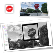
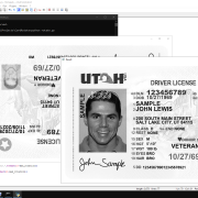
Another application of the problem explained in the article “Discovering a small image inside a large image using Python and OpenCV” is that you can use this code to find a special sign in a ID card Scan and make certain changes based on that.

For example, here we have given the program a type of sample certificate that has been scanned in reverse, and after finding the sign in the upper right corner of the card, we rotate it as many times as necessary to show the certificate image in the right direction.

Sample code:

import cv2

def find_image_in_larger_image(small_image, large_image):

# Read images

# Check if images are loaded successfully

if small_image is None or large_image is None:

print(“Error: Unable to load images.”)

return None

# Get dimensions of both images

small_height, small_width = small_image.shape

large_height, large_width = large_image.shape

# Find the template (small image) within the larger image

result = cv2.matchTemplate(large_image, small_image, cv2.TM_CCOEFF_NORMED)

# Define a threshold to consider a match

threshold = 0.6

# Find locations where the correlation coefficient is greater than the threshold

locations = cv2.findNonZero((result >= threshold).astype(int))

# If no match is found

if locations is None:

return None

# Determine the position of the matched areas

matched_positions = []

for loc in locations:

x, y = loc[0]

if x < large_width / 2:

position_x = “left”

otherwise:

position_x = “right”

if y < large_height / 2:

position_y = “top”

otherwise:

position_y = “bottom”

matched_positions.append((position_x, position_y))

return matched_positions

# Example usage

small_image_path = “mark.jpg”

large_image_path = “card.jpg”

small_image = cv2.imread(small_image_path, cv2.IMREAD_GRAYSCALE)

large_image = cv2.imread(large_image_path, cv2.IMREAD_GRAYSCALE)

rotated_large_image=large_image

positions = find_image_in_larger_image(small_image, large_image)

max_rotation = 10 # Set the maximum rotation limit

if positions:

position_x, position_y = positions[0]

print(“Position: {}, {}”.format(position_x, position_y))

while max_rotation>0:

max_rotation-=1

rotated_large_image = cv2.rotate(rotated_large_image, cv2.ROTATE_90_CLOCKWISE)

positions = find_image_in_larger_image(small_image, rotated_large_image)

if positions:

position_x, position_y = positions[0]

print(“Position: {}, {}”.format(position_x, position_y))

if(position_x==’right’ and position_y==’top’):

cv2.imshow(“Mark”, small_image)

cv2.imshow(“Original”, large_image)

cv2.imshow(“Result”, rotated_large_image)

cv2.waitKey(0)

cv2.destroyAllWindows()

max_rotation=0

otherwise:

print(“No match found after {} rotations.”.format(10-max_rotation))

otherwise:

print(“No match found after {} rotations.”.format(10-max_rotation))

Click here to view on GitHub.

Finding a Small Image Within a Larger Image Using Python and OpenCV

In this post, we’ll explore an interesting application of image processing using the Python programming language and the OpenCV library. The topic of this post is finding a small image within a larger image. This application can be used for pattern recognition, image matching, or even face detection.

First, make sure that OpenCV is installed in your Python environment. If you haven’t installed it yet, you can do so using the following commands:

pip install opencv-python
pip install opencv-python-headless


Now that OpenCV is installed, let’s delve into the Python code for finding an image within an image. The following code accomplishes this task:

import cv2

def find_image_in_larger_image(small_image_path, large_image_path):
# Read images
small_image = cv2.imread(small_image_path, cv2.IMREAD_GRAYSCALE)
large_image = cv2.imread(large_image_path, cv2.IMREAD_GRAYSCALE)

# Check if images are loaded successfully
if small_image is None or large_image is None:
print(“Error: Unable to load images.”)
return None

# Get dimensions of both images
small_height, small_width = small_image.shape
large_height, large_width = large_image.shape

# Find the template (small image) within the larger image
result = cv2.matchTemplate(large_image, small_image, cv2.TM_CCOEFF_NORMED)

# Define a threshold to consider a match
threshold = 0.8

# Find locations where the correlation coefficient is greater than the threshold
locations = cv2.findNonZero((result >= threshold).astype(int))

# If no match is found
if locations is None:
print(“No match found.”)
return None

# Draw rectangles around the matching areas
for loc in locations:
top_left = loc[0]
bottom_right = (top_left[0] + small_width, top_left[1] + small_height)
cv2.rectangle(large_image, top_left, bottom_right, (0, 255, 0), 2)

# Display the result (optional)
cv2.imshow(“Result”, large_image)
cv2.waitKey(0)
cv2.destroyAllWindows()

return locations

# Example usage
small_image_path = “small_image.jpg”
large_image_path = “large_image.jpg”

find_image_in_larger_image(small_image_path, large_image_path)

This code finds occurrences of the small image within the larger image and draws rectangles around the matching areas.

By running this code and replacing "small_image.jpg" and "large_image.jpg" with the paths to your actual images, you can experience its functionality.

Understanding Histogram of Oriented Gradients (HOG) for Face Detection

Introduction

In the realm of computer vision, face detection serves as a crucial task with applications spanning from security and surveillance to photography and social media. One powerful technique employed for object detection, including faces, is the Histogram of Oriented Gradients (HOG). In this article, we will explore the principles behind HOG, its methodology, and its implementation in Python using the OpenCV library.

The Basics of HOG

What is HOG?

HOG is a feature descriptor that captures the distribution of intensity gradients in an image. Developed by Navneet Dalal and Bill Triggs in 2005, HOG has proven to be highly effective in object detection tasks, particularly for detecting pedestrians and faces.

How Does HOG Work?

HOG operates on the premise that the local shape and appearance of an object can be characterized by the distribution of intensity gradients or edge directions. By dividing an image into small, overlapping cells, HOG computes the gradient orientation within each cell and creates histograms of these orientations. These histograms are then concatenated to form a feature vector, which serves as a representation of the object’s appearance.

Steps in HOG Computation:

  1. Gradient Computation:
    • Calculate the gradient of the image using techniques like Sobel operators to identify edges.
  2. Cell Division:
    • Divide the image into small cells to capture local gradient information.
  3. Histogram Calculation:
    • Compute histograms of gradient orientations within each cell.
  4. Block Normalization:
    • Normalize groups of cells, known as blocks, to account for changes in lighting and contrast.
  5. Feature Vector Formation:
    • Concatenate the normalized block histograms to form the final feature vector.

Implementing HOG in Python

Now, let’s dive into the practical aspect of HOG using Python and OpenCV. The following Python script demonstrates HOG-based face detection:

import cv2

# Load the image
image = cv2.imread(‘path/to/your/image.jpg’)

# Convert the image to grayscale
gray_image = cv2.cvtColor(image, cv2.COLOR_BGR2GRAY)

# Create a HOG face detector
hog_face_detector = cv2.HOGDescriptor()
hog_face_detector.setSVMDetector(cv2.HOGDescriptor_getDefaultPeopleDetector())

# Detect faces in the image using HOG
faces_hog, _ = hog_face_detector.detectMultiScale(gray_image)

# Draw bounding boxes around detected faces
for (x, y, w, h) in faces_hog:
cv2.rectangle(image, (x, y), (x + w, y + h), (0, 0, 255), 2)

# Display the image with bounding boxes
cv2.imshow(‘HOG Face Detection’, image)
cv2.waitKey(0)
cv2.destroyAllWindows()


Considerations and Tips

Parameters Tuning:

HOG-based detectors often have parameters that can be tuned for better performance. Experiment with parameters such as the scale factor and the minimum size of detected objects to achieve optimal results for your specific use case.

Computational Efficiency:

One of the strengths of HOG is its computational efficiency, making it suitable for real-time applications. However, the size of the detection window and the complexity of the image can impact processing time.

Limitations:

While HOG is effective in many scenarios, it may struggle with certain challenges, such as variations in lighting conditions and complex backgrounds. Understanding these limitations is essential when choosing an appropriate method for your application.

Conclusion

Histogram of Oriented Gradients (HOG) has become a cornerstone in object detection, providing a robust and computationally efficient means to capture the essential features of objects within images. In the context of face detection, HOG proves to be a reliable and versatile technique.

By grasping the fundamental concepts behind HOG and experimenting with its implementation in Python, you can gain valuable insights into its capabilities and limitations. As with any computer vision technique, fine-tuning and customization are key to achieving optimal results for your specific use case.

In the next part of this series, we will explore another powerful face detection method, Multi-task Cascaded Convolutional Networks (MTCNN), providing a comprehensive understanding of various techniques available for this critical computer vision task. Stay tuned!

Face Detection with HOG and MTCNN

Exploring Face Detection Techniques: HOG vs. MTCNN

Face detection is a fundamental task in computer vision with applications ranging from security systems to social media. Two popular methods for face detection are Histogram of Oriented Gradients (HOG) and Multi-task Cascaded Convolutional Networks (MTCNN). In this blog post, we’ll delve into both techniques, providing an overview of their principles and showcasing Python code for each.

Histogram of Oriented Gradients (HOG)

Understanding HOG

HOG is a feature descriptor widely used for object detection. It works by analyzing the distribution of gradients in an image, making it particularly effective for detecting objects with distinct shapes and textures.

How it Works

The HOG algorithm divides an image into small, overlapping cells, computes the gradient orientation within each cell, and then creates a histogram of these orientations. These histograms are then concatenated to form the final feature vector, which is used for training a support vector machine (SVM) or another classifier.

Python Code Example

We’ll begin by exploring HOG-based face detection using OpenCV in Python. The provided code loads an image, applies the HOG detector, and draws bounding boxes around detected faces.

View on GitHub

Multi-task Cascaded Convolutional Networks (MTCNN)

Understanding MTCNN

MTCNN is a deep learning-based face detection model designed to handle various face orientations and scales. It consists of three stages: face detection, bounding box regression, and facial landmark localization.

How it Works

MTCNN operates in a cascaded manner, with each stage refining the results of the previous one. The first stage detects potential face regions, the second stage refines the bounding boxes, and the third stage locates facial landmarks. The combined information provides accurate face detection.

Python Code Example

Next, we’ll explore face detection using MTCNN with the help of the `mtcnn` library in Python. The code loads an image, applies the MTCNN detector, and displays the image with bounding boxes around detected faces.

View on GitHub

Choosing the Right Method

While both HOG and MTCNN are effective for face detection, each has its strengths and limitations. HOG is robust and computationally efficient, making it suitable for real-time applications. On the other hand, MTCNN excels in handling diverse face orientations and is well-suited for scenarios where faces may appear at different scales and angles.

In the accompanying Python code, we showcase how to implement both techniques and provide insights into their usage. Feel free to experiment with the code and explore which method best fits your specific use case.

Continue reading for a detailed walkthrough of the code, usage instructions, and a discussion on factors influencing detection accuracy.